Cellular automata (or CA for short) are a fascinating computational model. They consist of a lattice of stateful cells and a transition rule that updates the state of each cell as a function of its neighbourhood configuration. By applying this local rule synchronously over time, we see interesting dynamics emerge.
For example, here is the transition table of Rule 110 in a 1-dimensional binary CA:
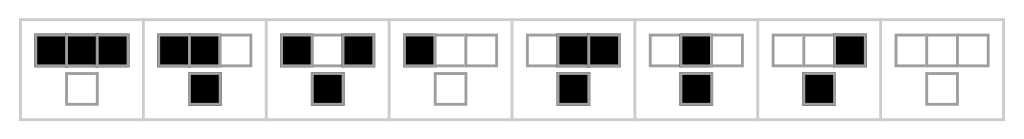
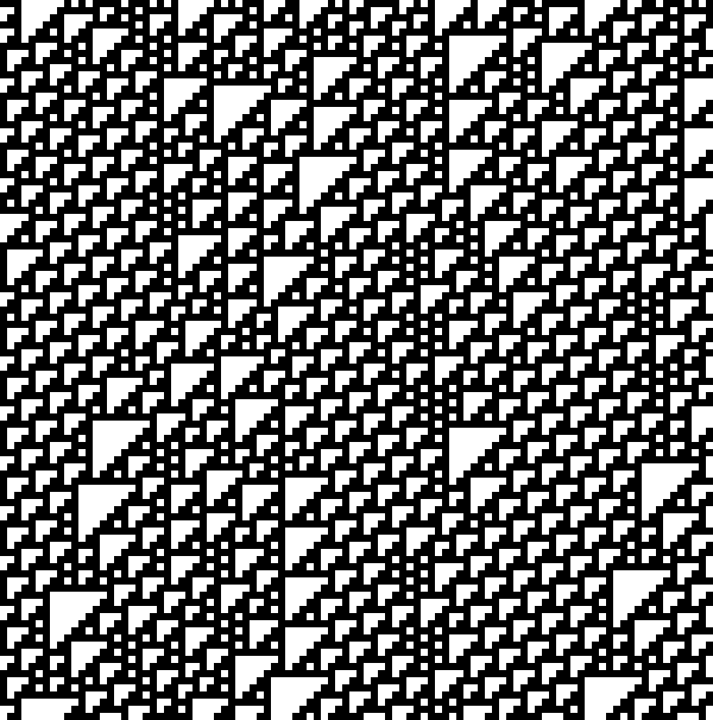
And here is the corresponding evolution of the states starting from a random initialization (time goes downwards):
By changing the rule, we get different dynamics, some of which can be extremely interesting. One example of this is the 2-dimensional Game of Life, with its complex patterns that replicate and move around the grid.
We can also bring this idea of locality to the extreme, by keeping it as the only requirement and making everything else more complicated.
For example, if we make the states continuous and change the size of the neighbourhood, we get the mesmerizing Lenia CA with its insanely life-like creatures that move around smoothly, reproduce, and even organize themselves into higher-order organisms.
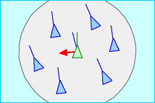
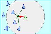
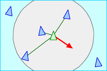
By this principle, we can also derive an even more general version of CA, in which the neighbourhoods of the cells no longer have a fixed shape and size. Instead, the cells of the CA are organized in an arbitrary graph.
Note that the central idea of locality that characterizes CA does not change at all: we’re just extending it to account for these more general neighbourhoods.
The super-general CA are usually called Graph Cellular Automata (GCA).
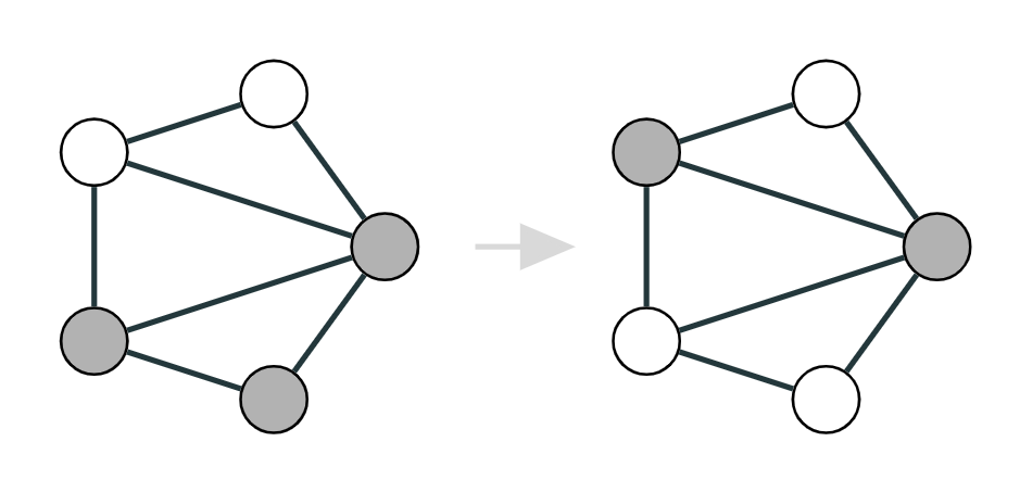
The general form of GCA transition rules is a map from a cell and its neighbourhood to the next state, and we can also make it anisotropic by introducing edge attributes that specify a relation between the cell and each neighbour.
Learning CA rules
The world of CA is fascinating, but unfortunately, they are almost always considered simply pretty things.
But can they be also useful? Can we design a rule to solve an interesting problem using the decentralized computation of CA?
The answer is yes, but manually designing such a rule may be hard. However, being AI scientists, we can try to learn the rule.
This is not a new idea.
We can go back to NeurIPS 1992 to find a seminal work on learning CA rules with neural networks (they use convolutional neural networks, although back then they were called “sum-product networks with shared weights”).
Since then, we’ve seen other approaches to learn CA rules, like these papers using genetic algorithms or compositional pattern-producing networks to find rules that lead to a desired configuration of states, a task called morphogenesis. Papers not on arXiv, sorry
More recently, convolutional networks have been shown to be extremely versatile in learning CA rules. This work by William Gilpin, for example, shows that we can implement any desired transition rule with CNNs by smartly setting their weights.
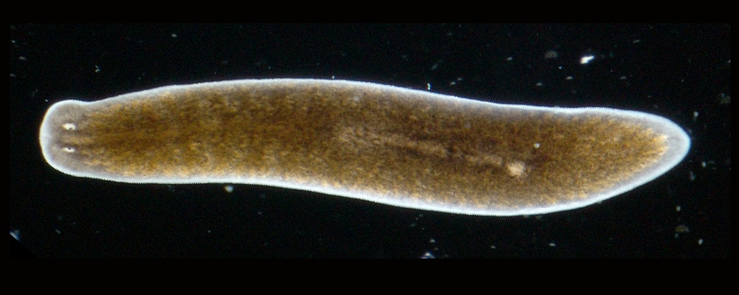
CNNs have also been used for morphogenesis. Inspired by the regenerative abilities of the flatworm (pictured above), in this visually-striking paper they train a CNN to grow into a desired image and to regenerate the image if it is perturbed.
Learning GCA rules
So, can we do something similar in the more general setting of GCA?
Well, let’s start with the model. Similar to how CNNs are the natural family of models to implement typical grid-based CA rules, the more general family of graph neural networks is the natural choice for GCA.
We call this setting the Graph Neural Cellular Automata (GNCA).
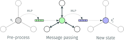
We propose an architecture composed of a pre-preprocessing MLP, a message-passing layer, and a post-processing MLP, which we use as transition function.
This model is universal to represent GCA transition rules. We can prove this by making an argument similar to the one for CNNs that I mentioned above.
I won’t go into the specific details here, but in short, we need to implement two operations:
- One-hot encoding of the states;
- Pattern-matching for the desired rule.
The first two blocks in our GNCA are more than enough to achieve this. The pre-processing MLP can compute the one-hot encoding, and by using edge attributes and edge-conditioned convolutions we can implement pattern matching easily.
Experiments
However, regardless of what the theory says, we want to know whether we can learn a rule in practice. Let’s try a few experiments.
Voronoi GCA
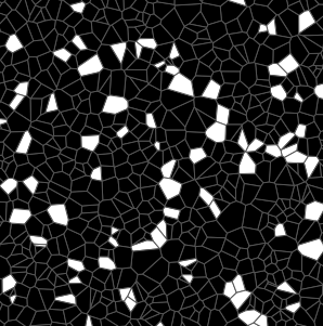
We can start from the simplest possible binary GCA, inspired by the 1992 NeurIPS paper I mentioned before. The difference is that our CA cells are the Voronoi tessellation of some random points. Alternatively, you can think of this GCA as being defined on the Delaunay triangulation of the points.
We use an outer-totalistic rule that swaps the state of a cell if the density of its alive neighbours exceeds a certain threshold, not too different from the Game of Life.
We try to see if our model can learn this kind of transition rule. In particular, we can train the model to approximate the 1-step dynamics in a supervised way, given that we know the true transition rule.


The results are encouraging. We see that the GNCA achieves 100% accuracy with no trouble and, if we let it evolve autonomously, it does not diverge from the real trajectory.
Boids
For our second experiment, we keep a similar setting but make the target GCA much more complicated. We consider the Boids algorithm, an agent-based model designed to simulate the flocking of birds. This can be still seen as a kind of GCA because the state of each bird (its position and velocity) is updated only locally as a function of its closest neighbours. However, this means that the states of the GCA are continuous and multi-dimensional, and also that the graph changes over time.
Again, we can train the GNCA on the 1-step dynamics. We see that, although it’s hard to approximate the exact behaviour, we get very close to the true system. The GNCA (yellow) can form the same kind of flocks as the true system (purple), even if their trajectories diverge.
Morphogenesis
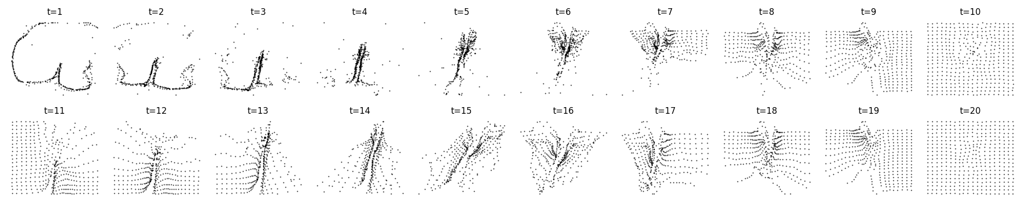
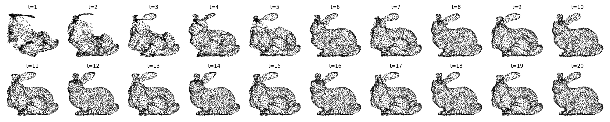
The final experiment is also the most interesting, and the one where we actually design a rule. Like previously in the literature, here too we focus on morphogenesis. Our task is to find a GNCA rule that, starting from a given initial condition, converges to a desired point cloud (like a bunny) where the connectivity of the cells has a geometrical/spatial meaning.
In this case, we don’t know the true rule, so we must train the model differently, by teaching it to arrive at the target state when evolving autonomously.
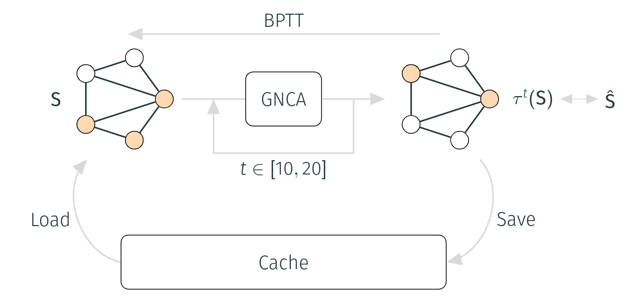
To do so, we let the model evolve for a given number of steps, then we compute the loss from the target, and we update the weights with backpropagation through time. To stabilise training, and to ensure that the target state becomes a stable attractor of the GNCA, we use a cache. This is a kind of replay memory from which we sample the initial conditions, so that we can reuse the states explored by the GNCA during training. Crucially, this teaches the model to remain at the target state when starting from the target state.
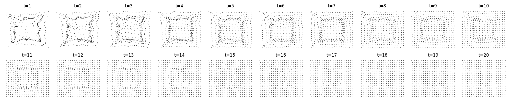
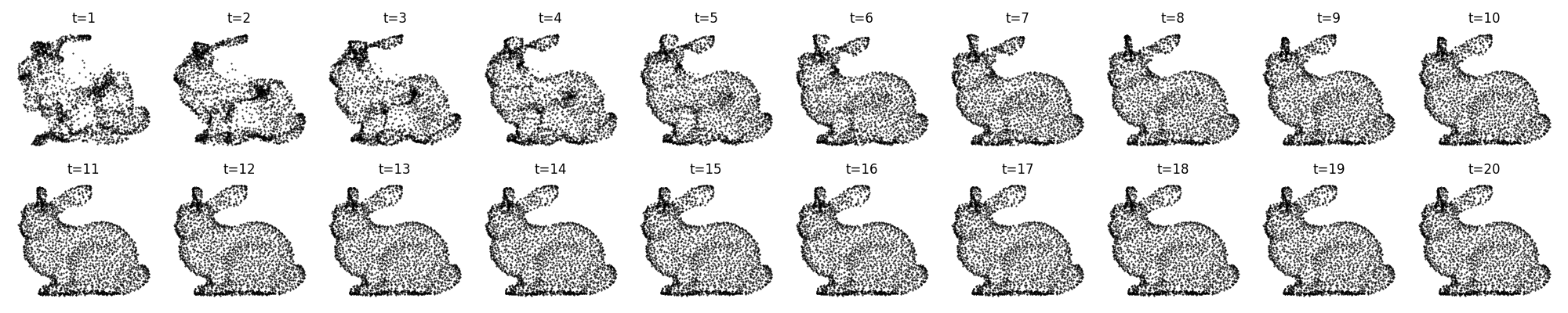
And the results are pretty amazing… have you seen the gif at the top of the post? Let’s unroll the first few frames here.
A 2-dimensional grid:
A bunny:
The PyGSP logo:
![]()
We see that the GNCA has no trouble in finding a stable rule that converges quickly at the target and then remains there.
Even for complex and seemingly random graphs, like the Minnesota road network, the GNCA can learn a rule that quickly and stably converges to the target:
However, this is not the full story. Sometimes, instead of converging, the GNCA learns to remain in an orbit around the target state, giving us these oscillating point clouds.
Grid:
Bunny:
Logo:
![]()
Now what?
So, where do we go from here?
We have seen that GNCA can reach global coherence through local computation, which is not that different from what we do in graph representation learning. In fact, the first GNN paper, back in 2005, already contained this idea.
But moving forward, it’s easy to see that the idea of emergent computation on graphs could apply to many scenarios, including swarm optimization and control, modelling epidemiological transmission, and it could even improve our understanding of complex biological systems, like the brain.
GNCA enable the design of GCA transition rules, unlocking the power of decentralised and emergent computation to solve real-world problems.
The code for the paper is available on Github and feel free to reach out via email if you have any questions or comments.
Read more
This blog post is the short version of our NeurIPS 2021 paper:
Learning Graph Cellular Automata
D. Grattarola, L. Livi, C. Alippi
You can cite the paper as follows:
@inproceedings{grattarola2021learning,
  title={Learning Graph Cellular Automata},
  author={Grattarola, Daniele and Livi, Lorenzo and Alippi, Cesare},
  booktitle={Neural Information Processing Systems},
  year={2021}
}