Mathematically modeling how epilepsy acts on the brain is one of the major topics of research in neuroscience. Recently I came across this paper by Oscar Benjamin et al., which I thought that it would be cool to implement and experiment with.
The idea behind the paper is simple enough. First, they formulate a mathematical model of how a seizure might happen in a single region of the brain. Then, they expand this model to consider the interplay between different areas of the brain, effectively modeling it as a network.
Single system
We start from a complex dynamical system defined as follows:
\[\dot{z} = f(z) = (\lambda - 1 + i \omega)z + 2z|z|^2 - z|z|^4\]where \( z \in \mathbb{C} \) and \(\lambda\) controls the possible attractors of the system.
For \( 0 < \lambda < 1 \), the system has two stable attractors: one fixed point and one attractor that oscillates with an angular velocity of \(\omega\) rad/s.
We can consider the stable attractor as a simplification of the brain in its resting state, while the oscillating attractor is taken to be the ictal state (i.e., when the brain is having a seizure).
We can also consider a noise-driven version of the system:
\[dz(t) = f(z)\,dt + \alpha\,dW(t)\]where \( W(t) \) is a Wiener process rescaled by a factor \( \alpha \).
A Wiener process \( W(t)_{t\ge0} \), sometimes called Brownian motion, is a stochastic process with the following properties:
- \(W(0) = 0\);
- the increments between two consecutive observations are normally distributed with a variance equal to the time between the observations:
In the noise-driven version of the system, it is guaranteed that the system will eventually escape any region of phase space, moving from one attractor to the other.
In short, we have a system that due to external, unpredictable inputs (the noise), will randomly switch from a state of rest to a state of oscillation, which we consider as a seizure.
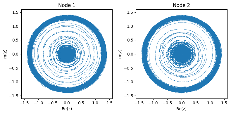
The two figures below show an example of the system starting from the stable attractor and then moving to the oscillator. Since the system is complex, we can observe its dynamics in phase space:
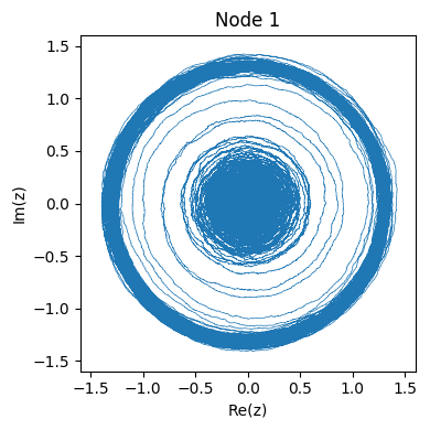
Or we can observe the real part of \( f(t) \) as if we were reading an EEG of brain activity:
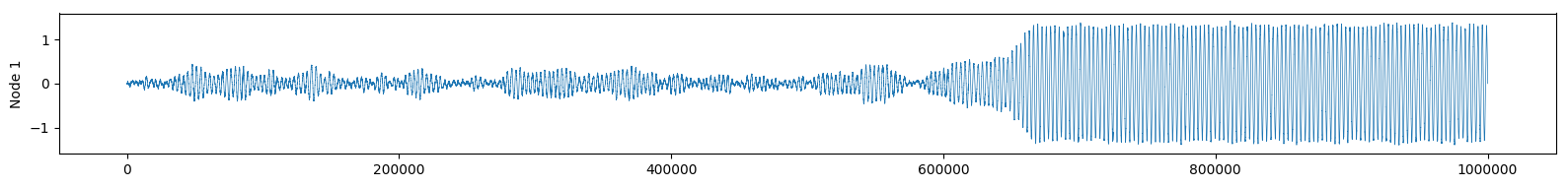
See how the change of attractor almost looks like an epileptic seizure?
Network model
While this simple model of seizure initiation is interesting on its own, we can also take our modeling a step further and explicitly represent the connections between different areas of the brain (or sub-systems, if you will) and how they might affect the propagation of seizures from one area to the other.
We do this by defining a connectivity matrix \( A \) where \( A_{ij} = 1 \) if sub-system \( i \) has a direct influence on sub-system \( j \), and \( A_{ij} = 0 \) otherwise. In practice, we also normalize the matrix by dividing each row element-wise by the product of the square roots of the node’s out-degree and in-degree.
Starting from the system described above, the dynamics of one node in the networked system are described by:
\[dz_{i}(t) = \big( f(z_i) + \beta \sum\limits_{j \ne i} A_{ji} (z_j - z_i) \big) + \alpha\,dW_{i}(t)\]If we look at the individual nodes, their behavior may not seem different than what we had with the single sub-system, but in reality, the attractors of these networked systems are determined by the connectivity \( A \) and the coupling strength \( \beta \).
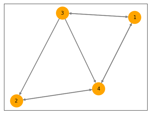
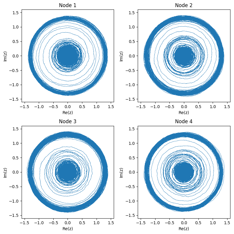
Here’s what the networked system of 4 nodes pictured above looks like in phase space:
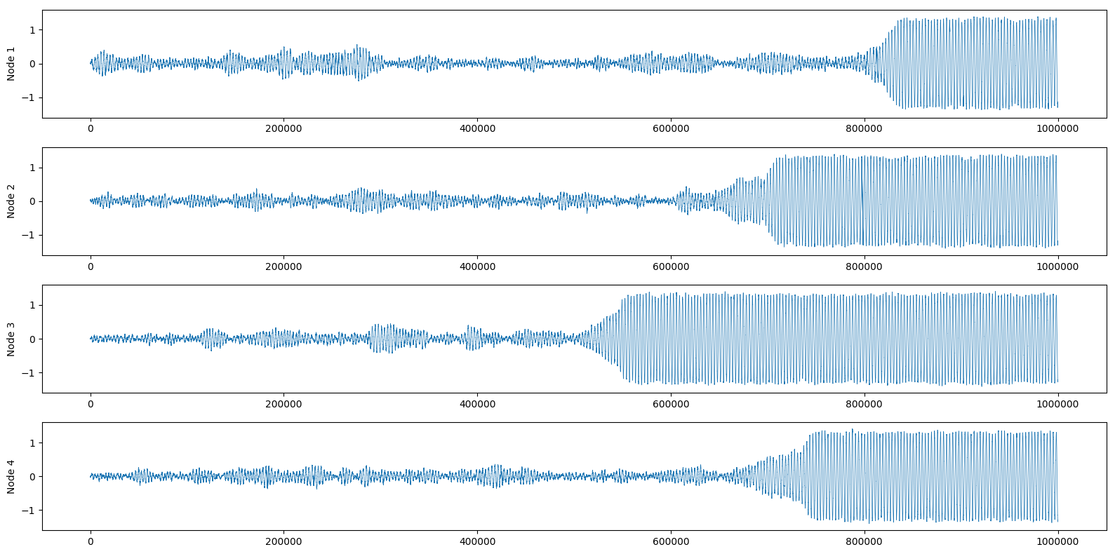
And again we can also look at the real part of each node:
If you want to have more details on how to control the different attractors of the system, I suggest you look at the original paper. They analyze in depth the attractors and escape times of all possible 2-nodes and 3-nodes networks, as well as giving an overview of higher-order networks.
Implementing the system with Numpy and Numba
Now that we got the math sorted out, let’s look at how to translate this system in Numpy.
Since the system is so precisely defined, we only need to convert the mathematical formulation into code. In short, we will need:
- The core functions to compute the complex dynamical system;
- The main loop to compute the evolution of the system starting from an initial condition.
While developing this, I quickly realized that my original, kinda straightforward implementation was painfully slow and that it would have required some optimization to be usable.
This was the perfect occasion to use Numba, a JIT compiler for Python that claims to yield speedups of up to two orders of magnitude.
Numba can be used to JIT compile any function implemented in pure Python, and natively supports a vast number of Numpy operations as well.
The juicy part of Numba consists of compiling functions in nopython mode, meaning that the code will run without ever using the Python interpreter.
To achieve this, it is sufficient to decorate your functions with the @njit decorator and then simply run your script as usual.
Code
At the very start, let’s deal with imports and define a couple of helper functions that we are going to use only once:
import numpy as np
from numba import njit

def degree_power(adj, pow):
    """
    Computes D^{p} from the given adjacency matrix.

    :param adj: rank 2 array.
    :param pow: exponent to which elevate the degree matrix.
    :return: the exponentiated degree matrix.
    """
    degrees = np.power(adj.sum(1), pow).reshape(-1)
    degrees[np.isinf(degrees)] = 0.
    D = np.diag(degrees)

    return D


def normalized_adjacency(adj):
    """
    Normalizes the given adjacency matrix using the degree matrix as
    D^{-1/2}AD^{-1/2} (symmetric normalization).

    :param adj: rank 2 array.
    :return: the normalized adjacency matrix.
    """
    normalized_D = degree_power(adj, -0.5)
    output = normalized_D.dot(adj).dot(normalized_D)

    return output
The code for these functions was copy-pasted from Spektral and slightly adapted so that we don’t need to import the entire library just for two functions. Note that there’s no need to JIT compile these two functions because they will run only once, and in fact, it is not guaranteed that compiling them will be less expensive than simply executing them with Python. Especially because both functions are heavily Numpy-based already, so they should run at C-like speed.
Moving forward to implementing the actual system. Let’s first define the fixed hyper-parameters of the model:
omega = 20               # Frequency of oscillations in rad/s
alpha = 0.2              # Intensity of the noise
lamb = 0.5               # Controls the possible attractors of each node
beta = 0.1               # Coupling strength b/w nodes
N = 4                    # Number of nodes in the system
seconds_to_generate = 1  # Number of seconds to evolve the system for
dt = 0.0001              # Time interval between consecutive states

# Random connectivity matrix
A = np.random.randint(0, 2, (N, N))
np.fill_diagonal(A, 0)
A_norm = normalized_adjacency(A).astype(np.complex128)
The core of the dynamical system is the update function \( f(z) \), that in code looks like this:
@njit
def f(z, lamb=0., omega=1):
    """The deterministic update function of each node.

    :param z: complex, the current state.
    :param lamb: float, hyper-parameter to control the attractors of each node.
    :param omega: float, frequency of oscillations in rad/s.
    """
    return ((lamb - 1 + complex(0, omega)) * z
            + (2 * z * np.abs(z) ** 2)
            - (z * np.abs(z) ** 4))
There’s not much to say here, except that using complex instead of np.complex seems to be slightly faster (157 ns vs. 178 ns), although the performance impact on the overall function is clearly negligible.
To compute the noise-driven system, we need to define the increment function of a complex Wiener process. We can start by implementing the increment function of a simple Wiener process, first:
@njit
def delta_wiener(size, dt):
    """Returns the random delta between two consecutive steps of a Wiener
    process (Brownian motion).

    :param size: tuple, desired shape of the output array.
    :param dt: float, time increment in seconds.
    :return: numpy array with shape 'size'.
    """
    return np.sqrt(dt) * np.random.randn(*size)
At the time of writing this, Numba does not support the size argument in np.random.normal but it does support np.random.randn. Instead of setting the scale parameter explicitly, we simply multiply the sampled values by the scale.
Since we are using the scale, and not the variance, we have to take the square root of the time increment dt.
Finally, we can compute the increment of a complex Wiener process as \( U(t) + jV(t) \), where both \( U \) and \( V \) are simple Wiener processes:
@njit
def complex_delta_wiener(size, dt):
    """Returns the random delta between two consecutive steps of a complex
    Wiener process (Brownian motion). The process is calculated as u(t) + jv(t)
    where u and v are simple Wiener processes.

    :param size: tuple, the desired shape of the output array.
    :param dt: float, time increment in seconds.
    :return: numpy array of np.complex128 with shape 'size'.
    """
    u = delta_wiener(size, dt)
    v = delta_wiener(size, dt)

    return u +  v * 1j
Now that we have all the necessary components to define the noise-driven system, let’s implement the main step function:
@njit
def step(z):
    """
    Compute one time step of the system, s.t. z[t+1] = z[t] + step(z[t]).

    :param z: numpy array of np.complex128, the current state.
    :return: numpy array of np.complex128.
    """
    # Matrix with pairwise differences of nodes
    delta_z = z.reshape(-1, 1) - z.reshape(1, -1)

    # Compute diffusive coupling
    diffusive_coupling = np.diag(A_norm.T.dot(delta_z))

    # Compute change in state
    update_from_self = f(z, lamb=lamb, omega=omega)
    update_from_others = beta * diffusive_coupling
    noise = alpha * complex_delta_wiener(z.shape, dt)
    dz = (update_from_self + update_from_others) * dt + noise

    return dz
Originally, I had implemented the following line
delta_z = z.reshape(-1, 1) - z.reshape(1, -1)
as
delta_z = z[..., None] - z[None, ...]
but Numba does not support adding new axes with None or np.newaxis.
Also, when computing diffusive_coupling, a more efficient way of doing
np.diag(A.T.dot(B))
would have been
np.einsum('ij,ij->j', A, B)
for reasons which I still fail to understand (3.48 µs vs. 2.57 µs, when A and B are 3 by 3 float matrices). However, Numba does not support np.einsum.
Finally, we can implement the main loop function that starts from a given initial state z0 and computes steps number of updates at time intervals of dt.
@njit
def evolve_system(z0, steps):
    """
    Evolve the system starting from the given initial state (z0) for a given
    number of time steps (steps).

    :param z0: numpy array of np.complex128, the initial state.
    :param steps: int, number of steps to evolve the system for.
    :return: list, the sequence of states.
    """
    steps_in_percent = steps / 100
    z = [z0]
    for i in range(steps):
        if not i % steps_in_percent:
            print(i / steps_in_percent, '%')
        dz = step(z[-1])
        z.append(z[-1] + dz)

    return z
I had originally wrapped the loop in a tqdm progress bar, but an old-fashioned if and print can reduce the overhead by 50% (2.29s vs. 1.23s, tested on a simple for loop with 1e7 iterations). Pre-computing steps_in_percent also reduces the overhead by 30% compared to computing it every time.
(You’ll notice that at some point it just became a matter of optimizing every possible aspect of this :D)
The only thing left to do is to evolve the system starting from a given intial state:
z0 = np.zeros(N).astype(np.complex128)  # Starting conditions
steps = int(seconds_to_generate / dt)   # Number of steps to generate

timesteps = evolve_system(z0, steps)
timesteps = np.array(timesteps)
You can now run any analysis on timesteps, which will be a Numpy array of np.complex128. Note also how we had to cast the initial conditions z0 to this dtype, in order to have strict typing in the JIT-compiled code.
I published the full code as a Gist, including the code I used to make the plots.
General notes on performance
My original implementation was based on a Simulator class that implemented all the same methods in a compact abstraction:
class Simulator(object):
    def __init__(self, N, A, dt=1e-4, omega=20, alpha=0.05, lamb=0.5, beta=0.1):
        ...

    @staticmethod
    def f(z, lamb=0., omega=1):
        ...

    @staticmethod
    def delta_weiner(size, dt):
        ...

    @staticmethod
    def complex_delta_weiner(size, dt):
        ...

    def step(self, z):
        ...

    def evolve_system(self, z0, steps):
        ...
There were some issues with this implementation, the biggest one being that it is much more messy to JIT compile an entire class with Numba (the substance of the code did not change much, and I’ve explicitly highlighted all implementation changes above).
Having moved to a more functional style feels cleaner and it honestly looks more elegant (opinions, I know). Crucially, it also allowed me to optimize each function to work flawlessly with Numba.
After optimizing all that was optimizable, I tested the old code against the new one and the speedup was about 31x, going from ~8k iterations/s to ~250k iterations/s.
Most of the improvement came from Numba and removing the overhead of Python’s interpreter, but it must be said that the true core of the system is dealt with by Numpy. In fact, as we increase the number of nodes the bottleneck becomes the matrix multiplication in Numpy, eventually leading to virtually no performance difference between using Numba or not (verified for N=1000 - the 31x speedup was for N=2).
I hope that you enjoyed this post and hopefully learned something new, be it about models of the epileptic brain or Python optimization.
Cheers!