In our latest paper, we presented a new pooling method for GNNs, called MinCutPool, which has a lot of desirable properties as far as pooling goes:
- It’s based on well-understood theoretical techniques for node clustering;
- It’s fully differentiable and learnable with gradient descent;
- It depends directly on the task-specific loss on which the GNN is being trained, but …
- It can be trained on its own without a task-specific loss if needed;
- It’s fast;
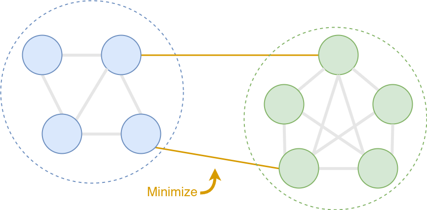
The method is based on the minCUT optimization problem, which consists of finding a cut on a weighted graph in such a way that the overall weight of the cut is minimized. We considered a continuous relaxation of the minCUT problem and implemented it as a neural network layer to provide a sound pooling method for GNNs.
In this post, I’ll describe the working principles of minCUT pooling and show some applications of the layer.
Background
The K-way normalized minCUT is an optimization problem to find K clusters on a graph by minimizing the overall intra-cluster edge weight. This is equivalent to solving:
\[\text{maximize} \;\; \frac{1}{K} \sum_{k=1}^K \frac{\sum_{i,j \in \mathcal{V}_k} \mathcal{E}_{i,j} }{\sum_{i \in \mathcal{V}_k, j \in \mathcal{V} \backslash \mathcal{V}_k} \mathcal{E}_{i,j}},\]where \(\mathcal{V}\) is the set of nodes, \(\mathcal{V_k}\) is the \(k\)-th cluster of nodes, and \(\mathcal{E_{i, j}}\) indicates a weighted edge between two nodes.
If we define a cluster assignment matrix \(C \in \{0,1\}^{N \times K}\), which maps each of the \(N\) nodes to one of the \(K\) clusters, the problem can also be re-written as:
\[\text{maximize} \;\; \frac{1}{K} \sum_{k=1}^K \frac{C_k^T A C_k}{C_k^T D C_k}\]where \(A\) is the adjacency matrix of the graph, and \(D\) is the diagonal degree matrix.
While finding the optimal minCUT is an NP-hard problem, there exist relaxations that can find near-optimal solutions in polynomial time. These relaxations, however, are still very expensive and are not able to generalize to unseen samples.
MinCUT pooling
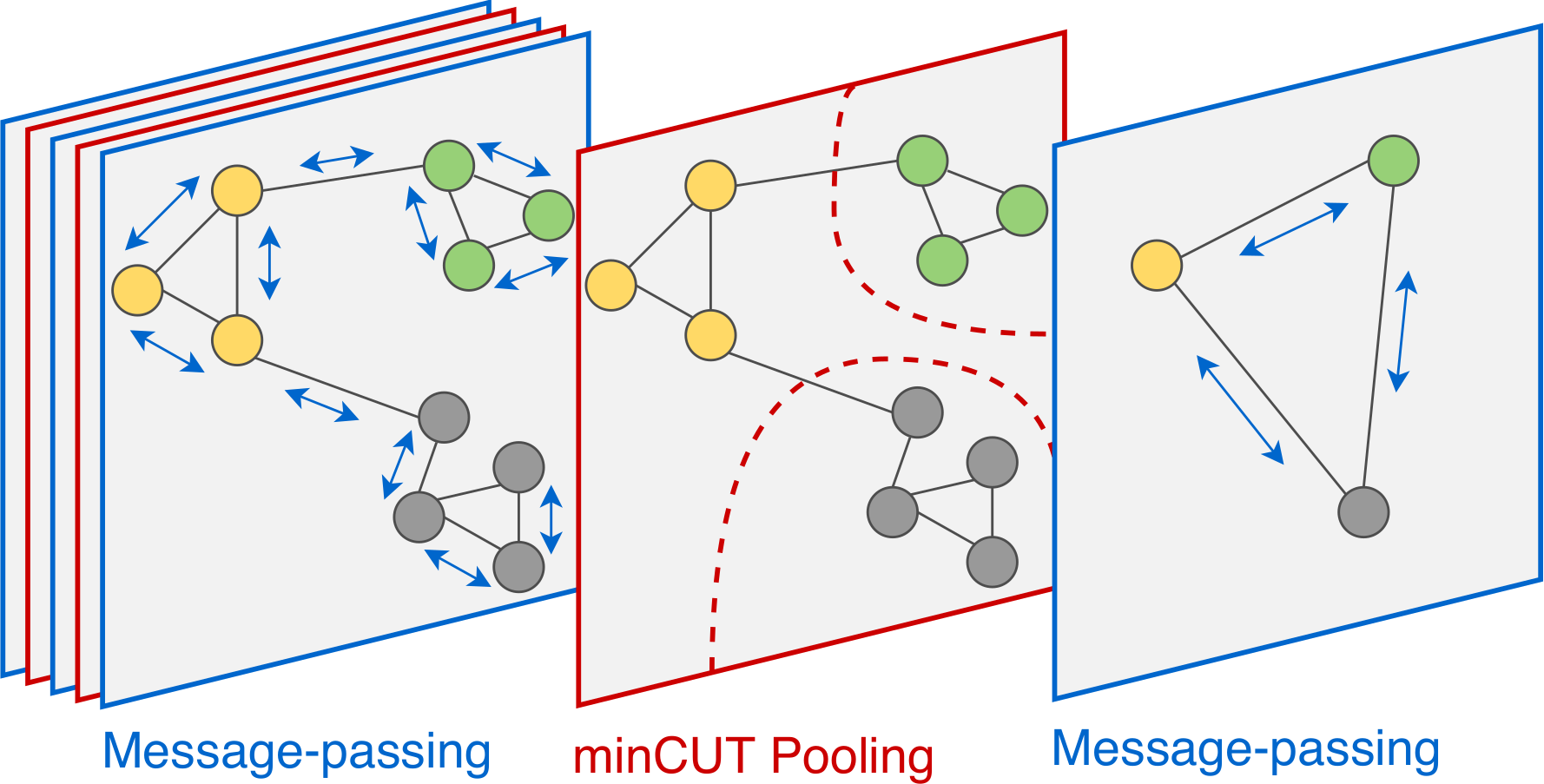
The idea behind minCUT pooling is to take a continuous relaxation of the minCUT problem and implement it as a GNN layer with a custom loss function. By minimizing the custom loss, the GNN learns to find minCUT clusters on any given graph and aggregates the clusters to reduce the graph’s size.
At the same time, because the layer can be used as a part of a larger architecture, any other loss that is being minimized during training will influence the clusters found by MinCutPool, making them optimal for the particular task at hand.
At the core of minCUT pooling there is a MLP, which maps the node features \(\mathbf{X}\) to a continuous cluster assignment matrix \(\mathbf{S}\) (of size \(N \times K\)):
\[\mathbf{S} = \textrm{softmax}(\text{ReLU}(\mathbf{X}\mathbf{W}_1)\mathbf{W}_2)\]We can then use the MLP to generate \(\mathbf{S}\) on the fly, and reduce the graphs with simple multiplications as:
\[\mathbf{A}^{pool} = \mathbf{S}^T \mathbf{A} \mathbf{S}; \;\;\; \mathbf{X}^{pool} = \mathbf{S}^T \mathbf{X}.\]At this point, we can already make a couple of considerations:
- Nodes with similar features will likely belong to the same cluster because they will be “classified” similarly by the MLP. This is especially true when using message-passing layers before pooling, since they will cause the node features of connected nodes to become similar;
- Because of the MLP, \(\mathbf{S}\) is pretty fast to compute and the layer can generalize to new graphs once it has been trained.
This is already pretty good, and it covers some of the main desiderata of a GNN layer, but we also want to explicitly account for the connectivity of the graph in order to pool it.
This is where the minCUT optimization comes in.
By slightly adapting the minCUT formulation above, we can design an auxiliary loss to train the MLP, so that it will learn to solve the minCUT problem in an unsupervised way.
In practice, our unsupervised regularization loss encourages the MLP to cluster together nodes that are strongly connected with each other and weakly connected with the nodes in the other clusters.
The full unsupervised loss that we minimize in order to achieve this is:
\[\mathcal{L}_u = \mathcal{L}_c + \mathcal{L}_o = \underbrace{- \frac{Tr ( \mathbf{S}^T \mathbf{A} \mathbf{S} )}{Tr ( \mathbf{S}^T\mathbf{D} \mathbf{S})}}_{\mathcal{L}_c} + \underbrace{\bigg{\lVert} \frac{\mathbf{S}^T\mathbf{S}}{\|\mathbf{S}^T\mathbf{S}\|_F} - \frac{\mathbf{I}_K}{\sqrt{K}}\bigg{\rVert}_F}_{\mathcal{L}_o},\]where \(\mathbf{A}\) is the normalized adjacency matrix of the graph.
Let’s break this loss down and see how it works.
Cut loss
The first term, \(\mathcal{L}_c\), encourages the MLP to find cluster assignments that solve the minCUT problem (to see why, compare it with the minCUT maximization that I described above). We refer to this loss as the cut loss.
In particular, minimizing the numerator leads to clustering together nodes that are strongly connected on the graph, while the denominator prevents any of the clusters to be too small.
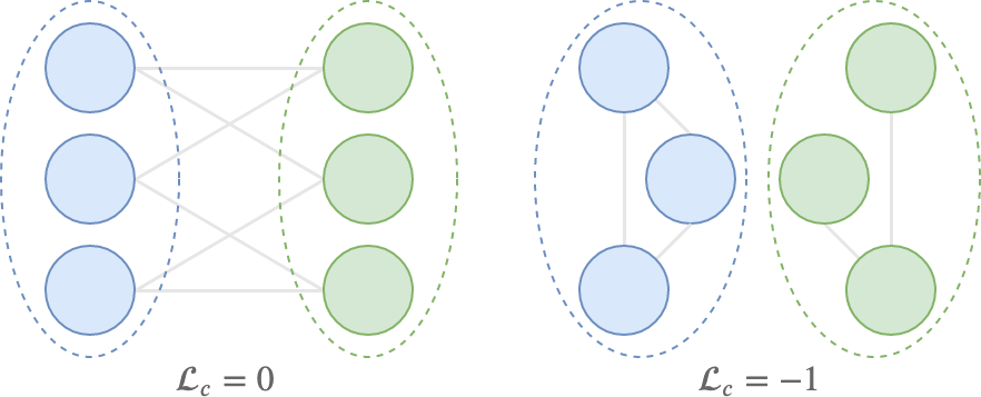
The cut loss is bounded between -1 and 0, which are ideally reached in the following situations:
- \(\mathcal{L}_c = 0\) when all pairs of connected nodes are assigned to different clusters;
- \(\mathcal{L}_c = -1\) when there are \(K\) disconnected components in the graph, and \(\mathbf{S}\) exactly maps the \(K\) components to the \(K\) clusters;
The figure below shows what these situations might look like. Note that both cases can only happen if \(\mathbf{S}\) is binary.
However, because of the continuous relaxation, \(\mathcal{L}_c\) is non-convex and there are spurious minima that can be found by SGD.
For example, for \(K = 4\), the uniform assignment matrix
would cause the numerator and the denominator of \(\mathcal{L}_c\) to be equal, and the loss to be \(-1\).
A similar situation occurs when all nodes in the graph are assigned to the same cluster.
This can be easily verified with Numpy:
In [1]: # Adjacency matrix
   ...: A = np.array([[1, 0, 1],
   ...:               [0, 1, 0],
   ...:               [1, 0, 1]])

In [2]: # Degree matrix
   ...: D = np.diag(A.sum(-1))

In [3]: # Perfect cluster assignment
   ...: S = np.array([[1, 0], [0, 1], [1, 0]])

In [4]: np.trace(S.T @ A @ S) / np.trace(S.T @ D @ S)
Out[4]: 1.0

In [5]: # All nodes uniformly distributed
   ...: S = np.ones((3, 2)) / 2

In [6]: np.trace(S.T @ A @ S) / np.trace(S.T @ D @ S)
Out[6]: 1.0

In [7]: # All nodes in the same cluster
   ...: S = np.array([[1, 0], [1, 0], [1, 0]])

In [8]: np.trace(S.T @ A @ S) / np.trace(S.T @ D @ S)
Out[8]: 1.0
Orthogonality loss
The second term, \(\mathcal{L}_o\), helps to avoid such degenerate minima of \(\mathcal{L}_c\) by encouraging the MLP to find clusters that are orthogonal between each other. We call this the orthogonality loss.
In other words, \(\mathcal{L}_o\) encourages the MLP to “make a decision” about which nodes belong to which clusters, avoiding those degenerate solutions where \(\mathbf{S}\) assigns one \(K\)-th of a node to each cluster.
Moreover, we can see that the perfect minimizer of \(\mathcal{L}_o\) is only reached if we have \(N \le K\) nodes, because in general, given a \(K\) dimensional vector space, we cannot find more than \(K\) mutually orthogonal vectors. The only way to minimize \(\mathcal{L}_o\) given \(N\) assignment vectors is, therefore, to distribute the nodes between the \(K\) clusters. This causes the MLP to avoid the other type of spurious minima of \(\mathcal{L}_c\), where all nodes are in a single cluster.
Interaction of the two losses
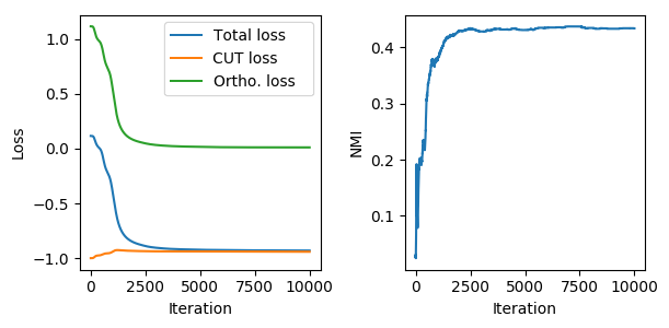
We can see how the two loss terms interact with each other to find a good solution to the cluster assignment problem. The figure above shows the evolution of the unsupervised loss as the network is trained to cluster the nodes of Cora (plot on the left). We can see that as the network is trained, the normalized mutual information (NMI) between the cluster assignments and the true labels improves, meaning that the layer is learning to find meaningful clusters (plot on the right).
Note how \(\mathcal{L}_c\) starts from a trivial assignment (-1) due to the random initialization and then moves away from the spurious minima as the orthogonality loss forces the MLP towards more sensible solutions.
Pooled graph
As a further consideration, we can take a closer look at the pooled adjacency matrix \(\mathbf{A}^{pool}\).
First of all, we can see that it is a \(K \times K\) matrix that contains the number of links connecting each cluster. For example, the entry \(\mathbf{A}^{pool}_{1,\;2}\) contains the number of links between the nodes in cluster 1 and cluster 2.
We can also see that the trace of \(\mathbf{A}^{pool}\) is being maximized in \(\mathcal{L}_c\). Therefore, we can expect the diagonal elements \(\mathbf{A}^{pool}_{i,\;i}\) to be much larger than the other entries of \(\mathbf{A}^{pool}\).
For this reason, \(\mathbf{A}^{pool}\) will represent a graph with very strong self-loops, and the message-passing layers after pooling will have a hard time propagating information on the graph (because the self-loops will keep sending the information of a node back onto itself, and not its neighbors).
To address this problem, a solution is to remove the diagonal of \(\mathbf{A}^{pool}\) and renormalize the matrix by its degree, before giving it as output of the pooling layer:
\[\hat{\mathbf{A}} = \mathbf{A}^{pool} - \mathbf{I}_K \cdot diag(\mathbf{A}^{pool}); \;\; \tilde{\mathbf{A}}^{pool} = \hat{\mathbf{D}}^{-\frac{1}{2}} \hat{\mathbf{A}} \hat{\mathbf{D}}^{-\frac{1}{2}}\]In the paper, we combined minCUT with message-passing layers that have a built-in skip connection, in order to bring each node’s information forward (e.g., Spektral’s GraphConvSkip). However, if your GNN is based on the graph convolutional networks (GCN) of Kipf & Welling, you may want to manually add the self-loops back after pooling.
Notes on gradient flow
The unsupervised loss \(\mathcal{L}_u\) can be optimized on its own, adapting the weights of the MLP to compute an \(\mathbf{S}\) that solves the minCUT problem under the orthogonality constraint.
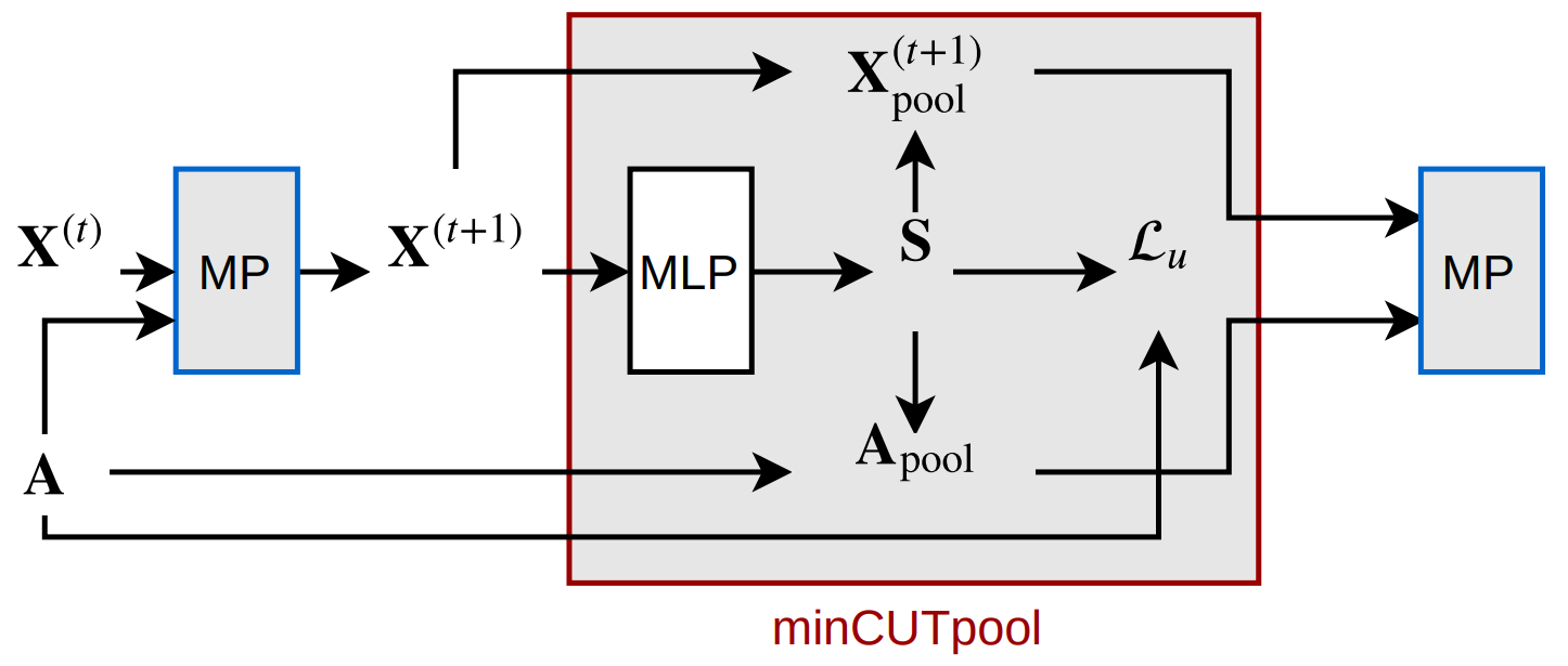
However, given the multiplicative interaction between \(\mathbf{S}\) and \(\mathbf{X}\), the gradient of the task-specific loss (i.e., whatever the GNN is being trained to do) can flow through the MLP. We can see in the picture above how there is a path going from the input \(\mathbf{X}^{(t+1)}\) to the output \(\mathbf{X}_{\textrm{pool}}^{(t+1)}\), directly passing through the MLP.
This means that the overall solution found by the GNN will keep into account both the graph structure (to solve minCUT) and the final task.
Code
Implementing minCUT in TensorFlow is fairly straightforward. Let’s start from some setup:
  import tensorflow as tf
  from tensorflow.keras.layers import Dense

  A  = ... # Adjacency matrix (N x N)
  X  = ... # Node features (N x F)
  n_clusters = ...  # Number of clusters to find with minCUT
First, the layer computes the cluster assignment matrix S by applying a softmax MLP to the node features:
H = Dense(16, activation='relu')(X)
S = Dense(n_clusters, activation='softmax')(H)  # Cluster assignment matrix
The cut loss is then implemented as:
# Cut loss
A_pool = tf.matmul(
  tf.transpose(tf.matmul(A, S)), S
)
num = tf.trace(A_pool)

D = tf.reduce_sum(A, axis=-1)
D_pooled = tf.matmul(
  tf.transpose(tf.matmul(D, S)), S
)
den = tf.trace(D_pooled)

mincut_loss = -(num / den)
And the orthogonality loss is implemented as:
# Orthogonality loss
St_S = tf.matmul(tf.transpose(S), S)
I_S = tf.eye(n_clusters)

ortho_loss = tf.norm(
    St_S / tf.norm(St_S) - I_S / tf.norm(I_S)
)
Finally, the full unsupervised loss of the layer is obtained as the sum of the two auxiliary losses:
total_loss = mincut_loss + ortho_loss
The actual pooling step is simply implemented as a simple multiplication of S with A and X, then we zero-out the diagonal of A_pool and re-normalize the matrix. Since we already computed A_pool for the numerator of \(\mathcal{L}_c\), we only need to do:
# Pooling node features
X_pool = tf.matmul(tf.transpose(S), X)

# Zeroing out the diagonal
A_pool = tf.linalg.set_diag(A_pool, tf.zeros(tf.shape(A_pool)[:-1]))  # Remove diagonal

# Normalizing A_pool
D_pool = tf.reduce_sum(A_pool, -1)
D_pool = tf.sqrt(D_pool)[:, None] + 1e-12  # Add epsilon to avoid division by 0
A_pool = (A_pool / D_pool) / tf.transpose(D_pool)
Wrap this up in a layer, and use the layer in a GNN. Done.
You can find minCUT pooling implementations both in Spektral and Pytorch Geometric.
Experiments
Unsupervised clustering
Because the core of MinCutPool is an unsupervised loss that does not require labeled data in order to be minimized, we can optimize \(\mathcal{L}_u\) on its own to test the clustering ability of minCUT.
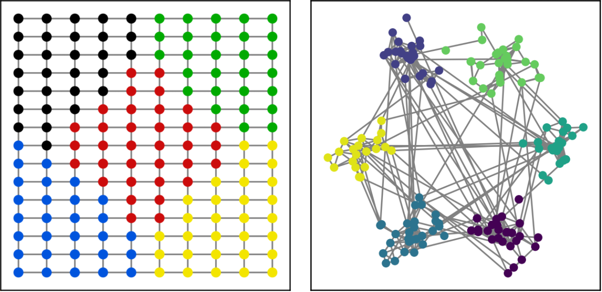
A good first test is to check whether the layer is able to cluster a grid (the size of the clusters should be the same) and to isolate communities in a network. We see in the figure below that minCUT was able to do this perfectly.
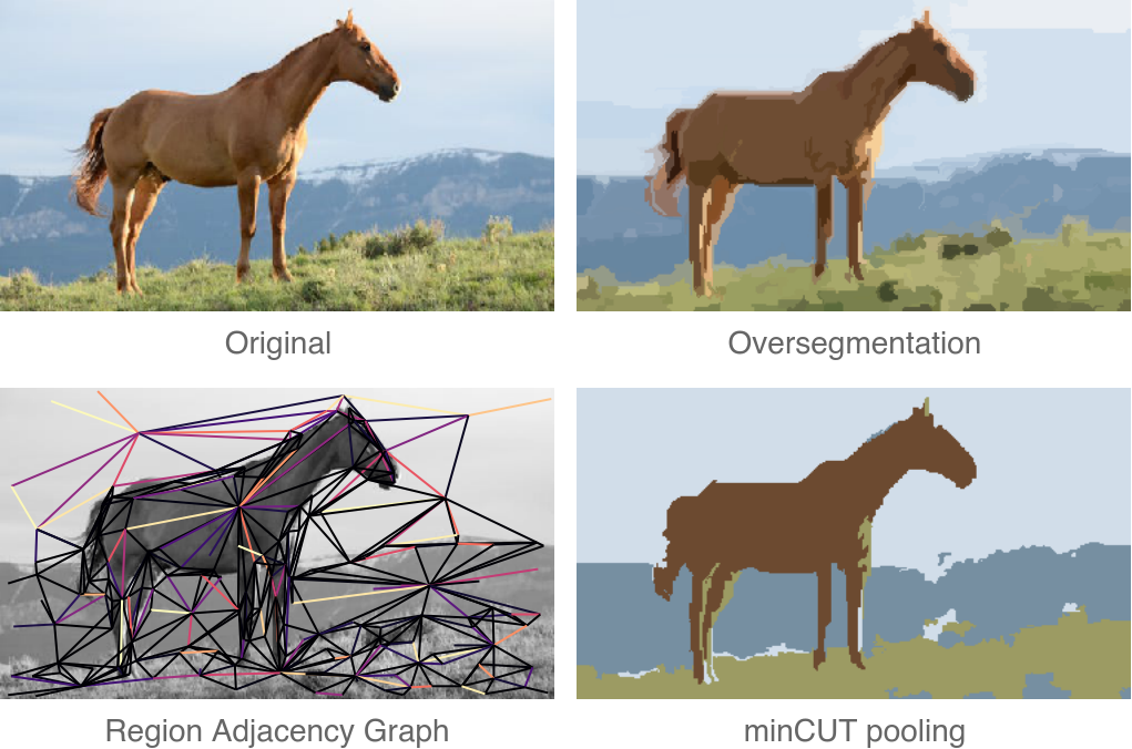
To make things more interesting, we can also test minCUT on the task of graph-based image segmentation. We can build a region adjacency graph from a natural image, and cluster its nodes in order to see if regions with similar colors are clustered together.
The results look nice, and remember that this was obtained by only optimizing \(\mathcal{L}_u\)!

Finally, we also checked the clustering abilities of MinCutPool on the popular citations datasets: Cora, Citeseer, and Pubmed. As mentioned before, we used the NMI score to see whether the layer was clustering together nodes of the same class. Note that the layer did not have access to the labels during training.
You can check the paper to see how minCUT fared in comparison to other methods, but in short: it did well, sometimes by a full order of magnitude better than other methods.
Autoencoder
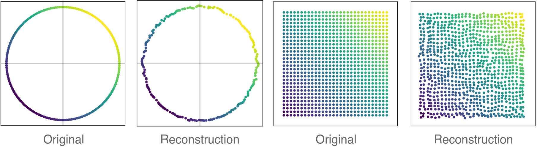
Another interesting unsupervised test that we did was to check how much information is preserved in the coarsened graph after pooling. To do this, we built a simple graph autoencoder with the structure pictured below:
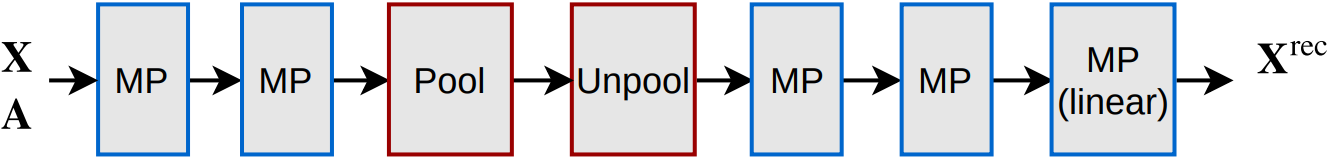
The “Unpool” layer is simply obtained by transposing the same \(\mathbf{S}\) found by minCUT, in order to upscale the graph instead of downscaling it:
\[\mathbf{A}^\text{unpool} = \mathbf{S} \mathbf{A}^\text{pool} \mathbf{S}^T; \;\; \mathbf{X}^\text{unpool} = \mathbf{S}\mathbf{X}^\text{pool}.\]We tested the graph AE on some very regular graphs that should have been easy to reconstruct after pooling. Surprisingly, this turned out to be a difficult problem for some pooling layers from the GNN literature. MinCUT, on the other hand, was able to defend itself quite nicely.
Supervised inductive tasks
Finally, we tested whether minCUT provides an improvement on the usual graph classification and graph regression tasks.
We picked a fixed GNN architecture and tested several pooling strategies by swapping the pooling layers in the network.
The dataset that we used were:
- The Benchmark Data Sets for Graph Kernels;
- A synthetic dataset created by F. M. Bianchi to test GNNs;
- The QM9 dataset for the prediction of chemical properties of molecules.
I’m not gonna report the comparisons with other methods, but I will highlight an interesting sanity check that we performed in order to see whether using GNNs and graph pooling even made sense at all.
Among the various methods that we tested, we also included:
- A simple MLP which did not exploit the relational information carried by the graphs;
- The same GNN architecture without pooling layers.
We were once again surprised to see that, while minCUT yielded a consistent improvement over such simple baselines, other pooling methods did not.
Conclusions
Working on minCUT pooling was an interesting experience that deepened my understanding of GNNs, and allowed me to see what is really necessary for a GNN to work.
We have put the paper on arXiv, and you can check the official implementations of the method in Spektral and Pytorch Geometric.
If you want to use MinCutPool in your own work, you can cite us with:
@article{bianchi2019mincut,
  title={Spectral Clustering with Graph Neural Networks for Graph Pooling},
  author={Filippo Maria Bianchi and Daniele Grattarola and Cesare Alippi},
  booktitle={Proceedings of the 37th International Conference on Machine learning (ICML)},
  year={2020}
}
Cheers!