When considering relational problems, the temporal dimension is often crucial to understand whether the process behind the relational graph is evolving, and how; think how often people follow and unfollow each other on Instagram, how the type of content in one’s posts may change over time, and how all of these aspects are echoed throughout the network, interacting with one another in complex ways.
While most works that apply deep learning to temporal networks are focused on the evolution of the graph at the node or edge level, it is extremely interesting to study a graph-based process from a global perspective, at the graph level, to detect trends and changes in the process itself.
This post is a simplified version of this paper, so you might want to have a look at either one before reading the other.
Be the change you want to see in the process
We consider a process generating a stream of graphs (e.g. hourly snapshots of a power supply grid), and we make the assumption of having two states: a nominal regime (when the grid is stable) and a non-nominal regime (when there’s about to be a blackout). We know what the graphs look like in the nominal state, and we can use a dataset of nominal graphs to train our models, but we cannot know what the non-nominal state will look like: the goal is to discriminate between the two regimes, regardless.
If we consider this as a one-class classification problem, then we have anomaly detection; if we take into account the temporal dimension, then the task is to detect whether the process has permanently shifted to non-nominal, and we have the change detection problem, on which we focus here.
Change detection can be easily formulated in statistical terms by considering two unknown nominal and non-nominal distributions driving a process, and running tests that can tell us whether the process is operating in one regime or the other.
When dealing with graphs, however, things get a bit more complicated.
While detecting changes in stationarity directly on the graph space is possible, it is also analytically complex. In particular, since most graph distances are non-metric, the resulting non-Euclidean geometry of the space is often unknown, making it quite harder to apply standard statistical tools. Even if we consider better-behaved metric distances, the computational complexity of dealing with the graph space is often intractable.
A common approach to circumvent this issue, then, is to represent the graphs in a simpler space via graph embedding.
Enter representation learning
The key idea behind our approach is the following: we train a graph autoencoder to extract a representation of the graphs on a somewhat simpler space, so that all the well known statistical tools for change detection become available for us to use.
However, since we already noted that graphs do not naturally lie in Euclidean spaces, we can look for a better embedding space, which can intrinsically represent some of the non-trivial properties of the space of graphs.
Since non-Euclidean geometry is basically any relaxation of the Euclidean one, we can freely pick our favorite non-Euclidean embedding space, where a desirable property of this space is to have computationally tractable metric distances, and a simple analytical form to make calculations easier.
A good family of spaces that reflect these characteristics is the family of constant curvature Riemannian manifolds (CCMs): hyperspheres and hyperboloids.
Algorithm overview
Let’s take a global view of the algorithm before diving into the details. The important steps are:
- Take a sequence of nominal graphs
- Train the AE to embed the graphs on a CCM
- Take a stream of graphs that may eventually change to the non-nominal regime
- Use the encoder to map the stream to the CCM
- Run a change detection test on the CCM to identify changes in the stream
The sequence of graphs in step 1 is also mapped to the CCM and used to configure the change detection test (more on that later).
In a real-world scenario, step 3 is the stream of graphs observed by the algorithm after being deployed, where we have no information on the real state of the system. To test our methodology, however, we consider a stream of graphs with a known change point, and use it as ground truth to evaluate performance.
Adversarial Graph Autoencoder
Building an autoencoder that maps the data distribution to a CCM requires imposing some sort of constraint on the latent space of the network, either by explicitly constraining the representation (e.g. by projecting the embeddings onto the CCM), or by letting the AE learn a representation on a CCM autonomously.
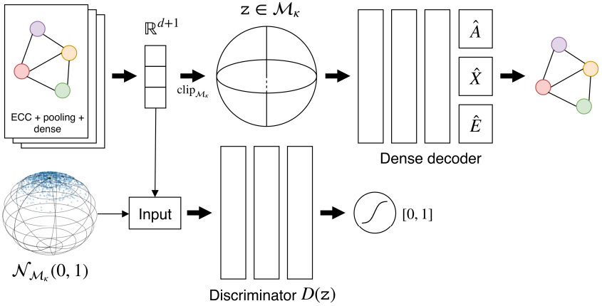
In our approach, we choose a mix of the two solutions: first, we let the AE learn a representation that lies as close as possible to the CCM, and then (once we’re sure that the projection will not introduce too much bias) we rectify the embeddings by clipping them onto the surface of the CCM.
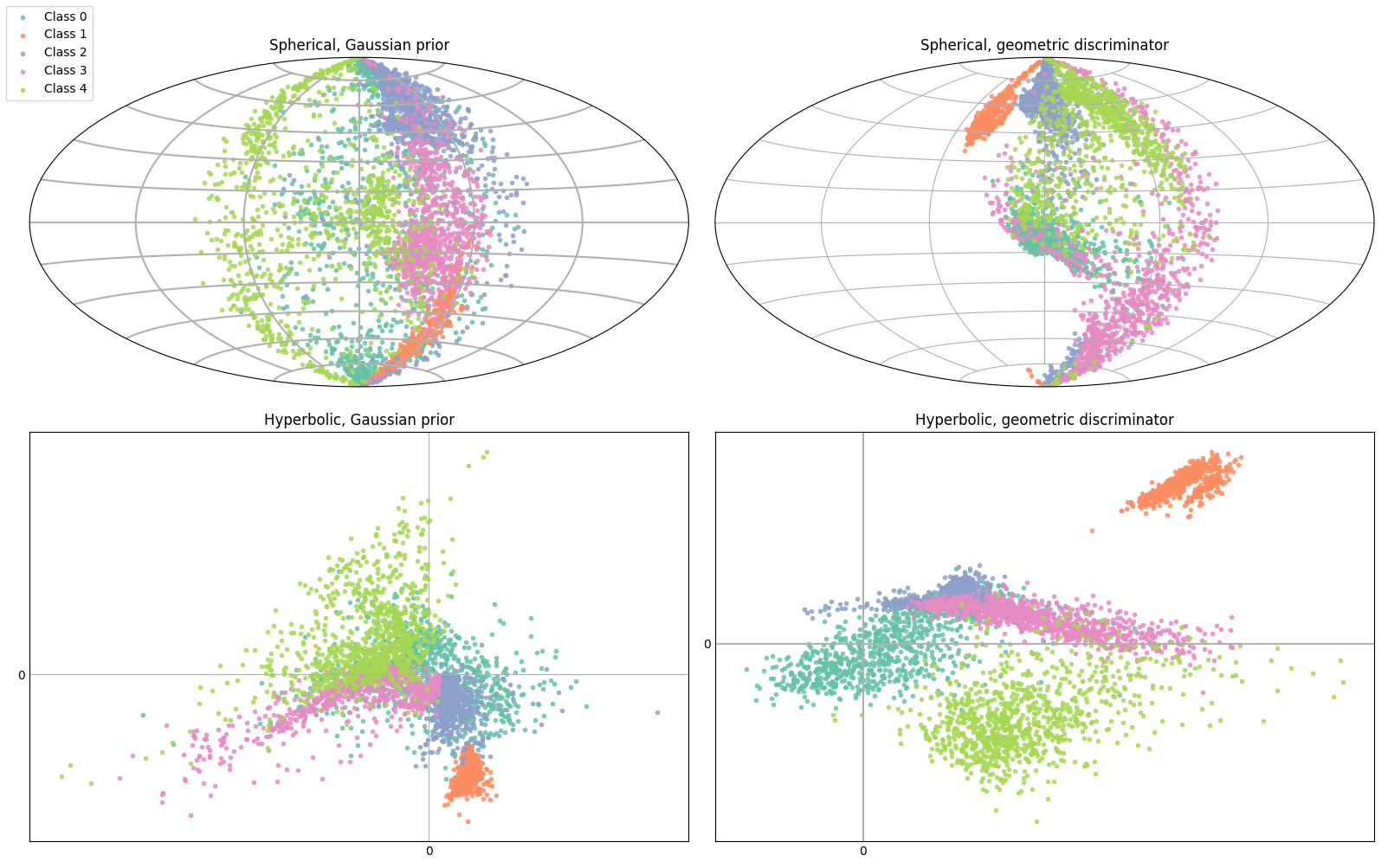
To impose an implicit constraint on the representation, we resort to the adversarial autoencoder framework, where we take a more GAN-like approach and only use the encoder as the generator, ignoring the decoder. We define a prior distribution with support on the CCM, by mapping an equivalent Euclidean distribution onto the CCM via the Riemannian exponential map, and we then match the aggregated posterior of the AE with this prior.
This has the twofold effect of 1) implicitly defining the embedding surface that the AE has to learn in order to confuse the discriminator network, and 2) making the AE use all of the latent space uniformly.
Using this CCM prior is the simplest modification to the standard AAE framework that we can make to impose the geometric constraint on the latent space, but in general we may want to drop the statistical conditioning of the posterior and find ways to let the AE learn the representation on the CCM freely. To do this, we introduce an analytical geometric discriminator.
Geometric discriminator
If we ignore the statistical conditioning of the AE’s posterior, we are left with the task of simply placing the embeddings onto the CCM. Since we already defined a training framework for the AE that relies on adversarial learning, we can stick to this methodology and slightly change it to fit our new, relaxed requirements.
The key idea behind adversarial networks is that both the generator and the discriminator strive to be better against each other, but what if the discriminator were already the best possible discriminator that may ever exist? What if the discriminator only had to compute a known classification function, without learning it?
This is the idea behind the geometric discriminator.
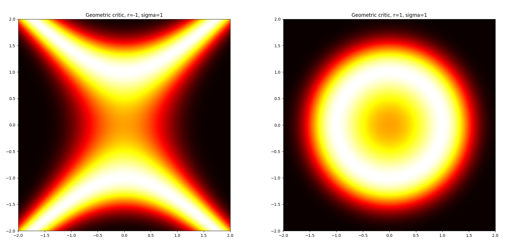
We consider a function \(D_\kappa(\vec z)\) depending on the curvature \(\kappa \ne 0\) of the CCM, where:
\[D_{\kappa}(\vec z) = \mathrm{exp}\left(\cfrac{-\big( \langle \vec z, \vec z \rangle - \frac{1}{\kappa} \big)^2}{2\varsigma^2}\right)\]which intuitively takes samples \(\vec z\) from the latent space and computes their membership to the CCM.
When optimized to fool the geometric discriminator, the AE will learn to place its codes on the CCM, while at the same time being free to choose the best latent representation to optimize the reconstruction loss.
In principle, we could argue that this formulation is equivalent to imposing a regularization term during the optimization of the AE, but experimental results showed us that separating the reconstruction and regularization phases yielded more stable and more effective results.
Change detection tests for CCMs
Having defined a way to represent our graph stream on a manifold with better geometrical properties than the simple Euclidean space, we now have to run the change detection test on the embedded stream of graphs.
Our change detection test is built upon the CUmulative SUMs algorithm (dating back to the 50’s), which basically consists in monitoring a generic stream of points by taking sequential windows of them, computing some local statistic across each window, and summing up the local statistics in a global accumulator.
The algorithm raises an alarm every time that the accumulator exceeds a particular detection threshold (and the accumulator is reset to 0 after that).
Using the (embedded) training graphs, we set the threshold such that the probability of the accumulator exceeding the threshold in the nominal regime is a given value \(\alpha\).
Once the threshold is set, we monitor the operational stream, knowing that any detection rate above \(\alpha\) will likely be associated to a change in the process.
Since the detection threshold is set by statistically studying the accumulator, we can estimate it by knowing the distribution of the local statistics that make up the accumulator. To do this, we consider as local statistic the Mahalanobis distance between the mean of the training samples and the mean of the operational window, which thanks to the central limit theorem has a known distribution.
So now we have outlined a change detection test for a generic stream, but where does non-Euclidean geometry come into play? In the paper we propose two different approaches to exploit it, both consisting in picking different ways to build the stream that is monitored by the CUSUM test.
Distance-based CDT (D-CDT): we take the training stream of nominal graphs and compute the Fréchet mean of the points on the CCM; for each embedding in the operational stream, then, we compute the geodesic distance between the mean and the embedding itself. This results in the stream of embeddings being mapped to a stream of distances, which we then monitor with the CUSUM-based algorithm described above.
Riemannian CLT-based CDT (R-CDT): here we take a slightly more geometrical approach, where instead of considering the Euclidean CLT we take the Riemannian CLT proposed by Bhattacharya and Lin, which works directly for points on a Riemannian manifold and modifies the Mahalanobis distance to deal with the non-Euclidean geometry. In short, the approach considers a stream of points obtained by mapping the CCM-embedded graphs to a tangent plane using the Riemannian log-map, and computes the detection threshold using the modified local statistic.
This might seem like a lot to deal with, but worry not: there’s a public repo to do this stuff for you.
Combined CCMs
As final touch, some considerations on what CCM to pick for embedding the graph stream.
In general, there are infinite curvatures to choose from, but we really only need to worry about the sign of the curvature, because that’s what determines whether the space is spherical or hyperbolic (or even Euclidean, if we set the curvature to 0).
Different problems may benefit from different geometries, depending on the task-specific distances that determine the geometry of the original space of graphs (for instance, MNIST - yes, images are graphs too - has been shown to do well on spherical manifolds).
But how can know whether a sphere or an hyperboloid is the best fit for a problem? How do we know that the Euclidean space isn’t actually the best one?
In principle, we could train an AE for each manifold and test the performance of the algorithm, but what if we don’t have enough data to get reliable results? What if have too much, and training is expensive?
A fairly trivial, but effective solution is to not pick just one manifold (pfffft!), but pick ALL of them at the same time and learn a joint representation.
Formally, we consider an ensemble manifold as the Cartesian product of different CCMs, and slightly adapt our architecture accordingly (essentially we take the relevant building blocks of our pipeline and put them in parallel, with some shared convolutions here and there - check Section 3.3 of the paper for details).
Since the actual values of the curvatures are less important than their signs, we can take only three CCMs to build our ensemble: a spherical CCM of curvature 1, an hyperbolic CCM of curvature -1, and an Euclidean CCM of curvature 0.
Experiments
To validate our methodology, we ran experiments in two different settings: a synthetic, controlled one, and a real-world scenario of epileptic seizure detection.
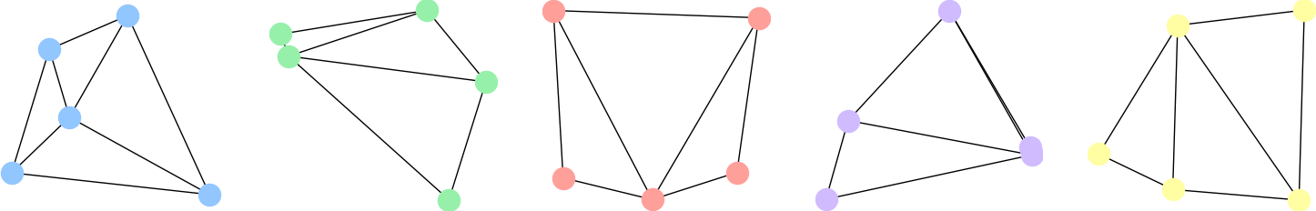
For the synthetic scenario, we considered graphs obtained as the Delaunay triangulations of points in a plane (pictured above), where we controlled the change in the stream by adding perturbations of different intensity to the support points of the graphs.
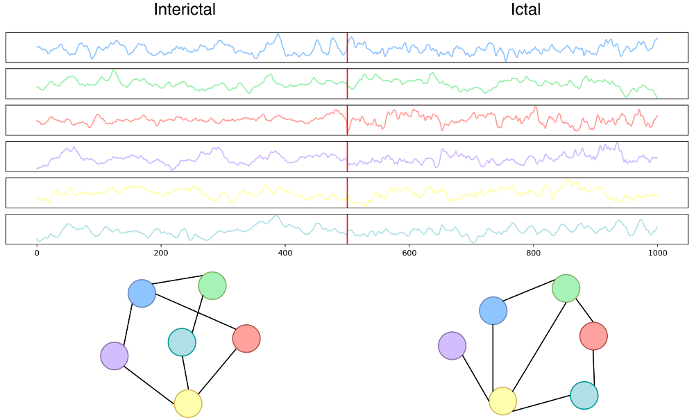
For the seizure detection scenario, we considered Kaggle’s UPenn and Mayo Clinic’s Seizure Detection Challenge and American Epilepsy Society Seizure Prediction Challenge datasets, composed of iEEG signals for different human and dog patients, with a different number of electrodes attached to each patient resulting in different multivariate signals.
The signals are provided in 1-second i.i.d. clips of different classes for each patient (the nominal interictal states where the patient is fine, and the non-nominal ictal states where the patient is having a seizure), and the original task of the challenge is to classify the clips correctly.
Since a common approach in neuroscience to deal with iEEG data is to build functional connectivity networks to study the relationships between different areas of the brain, especially during rare episodes like seizures, this task was the perfect playground to test our complex methodology.
We converted each 1-second clip to a graph using Pearson’s correlation as functional connectivity measure, and the topmost 4 wavelet coefficients of each signal as node attributes.
To simulate the graph streams, we used the labeled training data from the challenges to build the training and operational streams for each patient, where a change in the stream simply consisted in sampling graphs from the ictal class instead of the nominal.
Results in short
The important aspects that emerged after the experimental phase are the following:
- The ensemble of CCM, with the geometric critic, and R-CDT is the most effective change detection architecture among the ones tested (which included a purely Euclidean AE and a non-neural baseline for embedding graphs). This highlights how the AE is encoding different, yet useful information on the different CCMs;
- Exclusively spherical and hyperbolic AEs are relevant in some rare cases;
- Using the geometric discriminator often yields a better performance w.r.t. the standard discriminator, while reducing the number of trainable parameters by up to 13%;
- We are able to detect extremely small changes (in the order of \(10^{-3}\)) in the distribution driving the Delaunay stream;
- We are able to detect changes in both the iEEG detection and prediction challenges with good accuracy in most cases, except for a couple of patients for which we see an accuracy drop;
- The model does not require excessive hyperparameter tuning in order to perform well; a single configuration is good in most cases.
Conclusion
All methods introduces in this work can go beyond the limited application scenario that we reported in the paper.
Our aim was to introduce a new framework to deal with graphs on a global level, so as to make it possible to study the process underlying a graph-based problem as a whole.
The proposed techniques are modular and fairly generic: the adversarially regularized graph AE can be used to map graphs on CCMs for other tasks, and the embedding technique for CCMs can be used with other autoencoders and other data distributions. The change detection tests are a bit more specific, but represent a nice application of our new framework on relevant use cases.
We’re already working on new applications of this framework, to showcase what we believe to be a great potential, so stay tuned!
Credits
The code for replicating our experiments is available on my Github.
If you wish to reference our paper, you can cite:
@article{grattarola2018change,
  title={Change Detection in Graph Streams by Learning Graph Embeddings on Constant-Curvature Manifolds},
  author={Grattarola, Daniele and Zambon, Daniele and Livi, Lorenzo and Alippi, Cesare},
  journal={IEE Transactions on Neural Networks and Learning Systems},
  year={2019},
  doi={10.1109/TNNLS.2019.2927301}
}